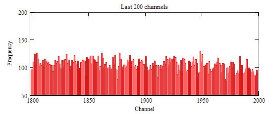
The number of channels that we want our compressed array to have
The number of channels of our raw arrray that will be in each channel of our compressed array
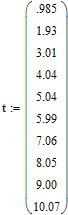
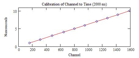
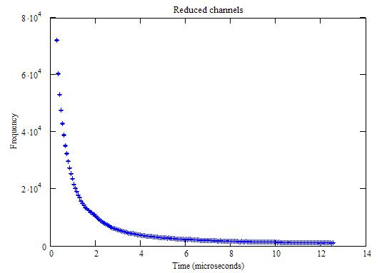
converting channels over to nanoseconds
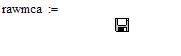
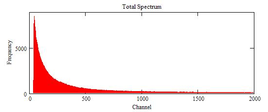
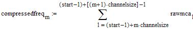
converting frequency to compressed frequency
creating upper and lower error limits for compressed frequency
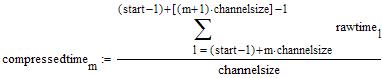
converting raw time to compressed time
creating upper and lower error limits for compressed time
A function to weight the points with respect to the error. We do this for six different weights, then examine results to determine which is the proper weight to use.
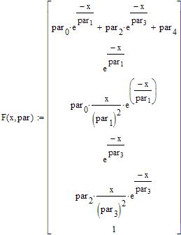
Creating vectors for the function fitting algorithm.
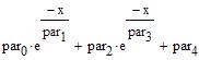
guess values for the parameters of:
Prof Decowski's parameters
Mathcad's algorithm for determining parameters
Mathcad's values of tfor each of the different weights.
Diagram 3: Weight Error Analysis
This seems to stabilize with an error weight of
, so using this error weight:
Mathcad's parameters
Diagram 4: Polonium-212 Half-life
OOO
Experimental points
___
Mathcad's parameters
___
Prof Decowski's parameters
Calculating the half life of 212Po (see diagram 6).
212Polonium has a half-life of 313 4 ns.
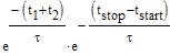
Diagram 5: OGC Delay Dependance on t
But
is just a constant so:
Therefore, the delay supplied by the OGC does not matter when solving for t.
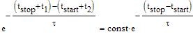
Diagram 6: Extracting the half-life () from t
but, in this case
. Therefore,
and
. Taking the inverse of both sides,
. Solving for
we find that:
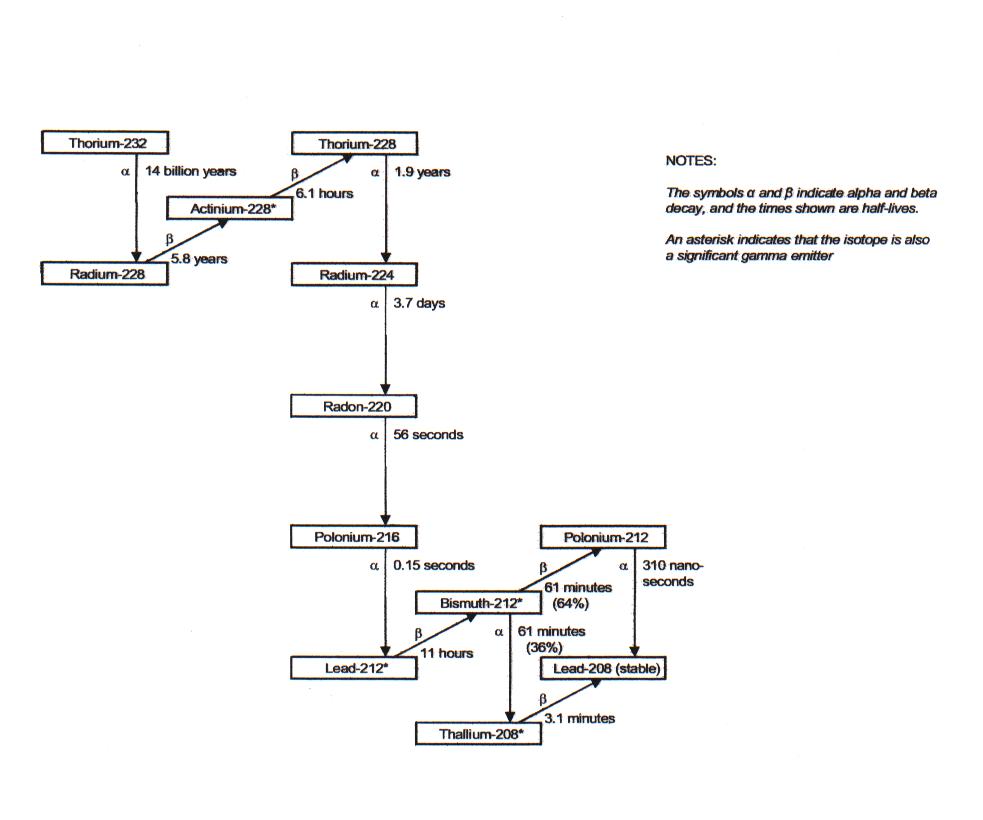
Diagram 7: Thorium-232 Decay Chain
From the Argonne National Laboratory at the University of Chicago, July 2002. http://www.ead.anl.gov/pub/doc/NaturalDecaySeries.pdf


 is just a constant so:
 but, in this case
 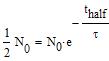 and
and  . Taking the inverse of both sides,
  . Solving for